Grey day. But, on the little Timber Trail up at the top of Highway 18 on Tiger Moutain, someone told me about the trail to Dirty Harry’s Balcony.
I’d wondered whether you could get to the top of any of the rock outcrops on the north side of I90 just east of North Bend.
Sure ’nuff.
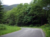
Turns out, you take Exit 38, the 1st exit east of North Bend. You gotta drive on the old road east a bit past a state park, then under the freeway. Then stop. There, you either go back on I90 westbound, or you take the neat little road up and around to the fire department training grounds. The sign says that they close the gate at 4pm. It’s 5 when I cruise in. Gate’s open.
I explore the road. Small signs along the way. E.g “Pick you heros carefully.” “You own your reaction.” Even without the occasional full sized pickups and anonymous fleet vans, you can guess that this road leads to a world where they play for keeps.
See the trailhead. Measure the distance back to outside the gate. 0.6 miles. Ok. Park outside the gate, stroll back up the road, across the little bridge, up the hill to the trailhead:
Google Maps Note: Google Earth has a much better picture and a Google Earth Community link to the trailhead.
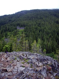
The trail is not a big thing. Just cuts off from the road – not as I think (apparently without a cap) straight back north toward Mailbox Peak, but rather, east up a steady, but unsteep slope.
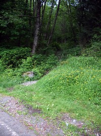
Anyway, the trail is one of these straight-up-the-wash things. Kinda rocky. OK, though. Eventually, it hangs a Louie. That’s where the cutoff is for the Balcony. There is a little coil of that 1-inch, rusted, stranded cable you see so often in the woods. And, someone put a little streamer on a bush.
I try to take a picture of the cutoff, but the batteries are dead. … Yank the spares out. … Ooops. They don’t even light up the camera to tell me the battery is dead. What a drag. That means I’ll have to come back sometime to shoot the rest of the trail’s sights. Well, that’s ok, ’cause the left turn has me wondering. Is it another way to get up Mailbox? That’d be quite cool. Go up from I90. Go down the other side to the road/trail up to Granite Lakes. Miss the main trail completely. A real gonzo path, that would be.
Anyway, I take the cutoff and in a few hundred yards of some up, some down, last up, pop out on the Balcony. Top of the rocks, looking at a swirly I90 going east. (The depleted batteries spring back to life for a couple of pictures.)
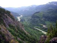
And, looking back up the rocks toward the east end of MailBox Peak:
It’s a bit humid. Close to the low clouds. And, I’ve run out of Kirkland Sport Drink so there’s no reason to linger. I head back.
A bit back on the trail – maybe 50 to 100 yards – there’s a cutoff to the east. Someone has put a branch over the cutoff trail to indicate that it’s the wrong trail. Coming up the trail, the right hand trail turns and goes up to the rocks. The right-turn trail feels right. But, the blocked trail looks interesting. Maybe it goes over to more of the rocks to the east. Let’s see.
I follow it. It’s a real trail. Not a freeway. Looks like maybe it’s a trail used by rock climbers. Up, down, up, up. Ladies, leave your high heels at home. This trail feels very nice.
Eventually, it comes out in one of those open groves of ceders and such. You know the kind. Lots of needles and brown stuff all over. No undergrowth. The trail could be just about anywhere, since the whole area is walkable. I’m thinking, “Hmmm. If this ends up being a longer trail than I’ve planned, I could be coming back here under the LED light.” That’s not good. Even in the best of times, I tend to wander off trails – accidentally or on purpose. Makes no difference. And, I know from harsh experience that I have a real hard time keeping to vague trails running through areas like this open area – in the light. In the dark, it’s random walk time.
Oh well. Getting off the trail isn’t a worry until later.
“Later” is in 2 minutes. The trail came from the upper left area of the grove and, according to my best estimate, peters out somewhere in the upper right area of the grove. What to do? Go back? By Jove, surely you jest!
There are two alternatives:
- Go to the edge of the open area and look for where the trail leaves.
- Start heading down.
It’s a cinch that the trail goes out of the area about 50 feet from where I am, so alternative 1 is the clear choice.
I choose 2.
Why? Well, if I go with 1, then I’ll pick up the trail, continue along it, and maybe, in about 11-teen miles, get to some other trail from I90. Hungry. Thirsty. Tired. A long way from the car. … Or, I’ll need to come back on this trail – and get lost in the clear grove.
If I go with 2, then I have a chance to come down off the hill in a completely different way than how I got up.
Down we go.
After all, in this kind of forest, the going is pretty good. No brambles to whack through.
I follow it down. … And down. … And down. … Oh, oh. Climbing back out of this thing is not an appealing prospect.
So, down we go some more.
Ah, I hear a stream. Good. Worst case, I can always follow the stream down to I90. Unless it goes over a waterfall. Then I’ll need to improvise.
Well, luck stays with the innocent.
Sure, it’s steady going through moss-on-rock-and-rotten-wood. And, sure, it’s one of those places where there is always a much clearer path about 20 to 50 feet to the left – or right – either one. Take your pick. They both look better than the raggity place you’re in.
Sure, after a couple of slips, I’m glad that I’m wearing old jeans rather than the nice, white pants I so often wear hiking.
No Tarzaning to be done, no vertical stuff, just easy going.
And, you can’t get lost on a steep hill aimed at the sound of Interstate Waterfall.
Score! No brambles at the bottom. Old, old road, completely overgrown by wildflowers. Little building of some sort connected to the shoulder of I90 by a dirt “road”.
Dang. No old road back to the car. Walking on freeways is no fun. Loud. Loud. And, gosh, cars really boogie along nowadays. Not like when we were kids.
And, woe is me:
Exit 38
1 Mile
That’s when I realize that my thinking about the direction of the main trail had been wrong. It was a long trudge back. Soaked pants and shirt from the mist and wet grass.
And, the Gold Honda has “emergency” clothes. So, I step in to ’em in under a light June rain.
The gate was still open at 7:30 as I drove away.
All in all, if you gotta dig in to your emergency gear, it’s been a great walk.
 Large image
 Large image
 Large image